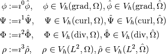
DeRham sequences
here without boundary conditions

Pullbacks
In the case where the physical domain  is the image of a logical domain
  by a smooth mapping
  (at least
  ), we have the following parallel diagrams
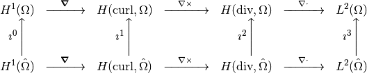
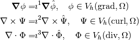
Where the mappings  and
and  are called pullbacks and are given by
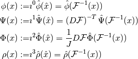
where  is the jacobian matrix of the mapping .
Note
The pullbacks and are isomorphisms between the corresponding spaces.
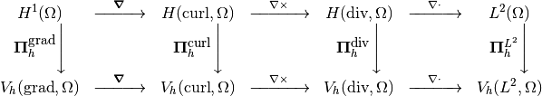
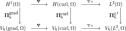
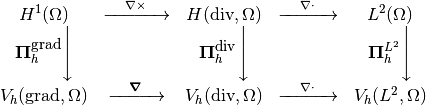
Discrete Spaces
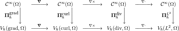
Let us suppose that we have a sequence of finite subspaces for each of the spaces involved in the DeRham sequence. The discrete DeRham sequence stands for the following commutative diagram between continuous and discrete spaces
When using a Finite Elements methods, we often deal with a reference element, and thus we need also to apply the pullbacks on the discrete spaces. In fact, we have again the following parallel diagram
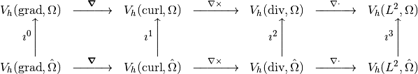
Since, the pullbacks are isomorphisms in the previous diagram, we can define a one-to-one correspondance
We have then, the following results
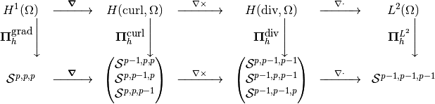
Discrete DeRham sequence for B-Splines
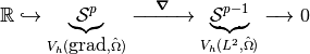
Buffa et al [BSV09] show the construction of a discrete DeRham sequence using B-Splines, (here without boundary conditions)
1d case
- DeRham sequence is reduced to
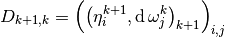
- The recursion formula for derivative writes

- we have
 which is a change of basis as a diagonal matrix
 - Now if
 , with and expansion
 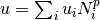 , we have
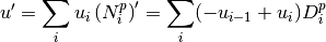
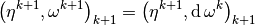
- If we introduce the B-Splines coefficients vector
 (and
(and  for the derivative), we have

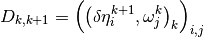
where  is the incidence matrix (of entries
  and
and  )
)
Discrete derivatives:

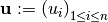
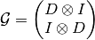
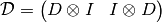
2d case
In 2d, the are two De-Rham complexes:
and
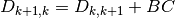
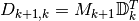
Let  be the identity matrix, we have
Discrete derivatives:
![\mathcal{C} =
\begin{pmatrix}
I \otimes D
\\
- D \otimes I
\end{pmatrix}
\quad \mbox{[scalar curl],} \quad
\mathcal{C} =
\begin{pmatrix}
- I \otimes D
&
D \otimes I
\end{pmatrix}
\quad \mbox{[vectorial curl]}](../_images/math/409e0105fb79c34ef7fc89a070283d24afc00575.png)
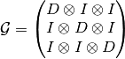
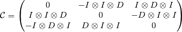
3d case
Discrete derivatives:

Note
From now on, we will denote the discrete derivative by  for the one going from
  to
to  .
.
Algebraic identities
Let us consider the discretization of the exterior derivative

multiplying by a test function  and integrating over the whole computation domain, we get
let  ,
,  and
and  be the vector representation of ,
  and
and  . We get

where
On the other hand, using the coderivative, we get

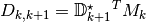
Let us now introduce the following matrix
hence,

Therefor, we have the following important result
Proposition:
References
| [BSV09] | A. Buffa, G. Sangalli, and R. Vazquez. Isogeometric analysis in electromagnetics: b-splines approximation. Comput. Methods Appl. Mech. Engrg, 199:1143–1152, 2009. |