B-Splines and NURBS
We start this section by recalling some basic properies about B-splines curves and surfaces. We also recall some fundamental algorithms (knot insertion and degree elevation).
For a basic introduction to the subject, we refer to the books [LP95] and [Far02].
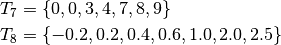
A B-Splines family,  of order
  , can be generated using a non-decreasing sequence of knots
 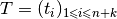 .
.
B-Splines series
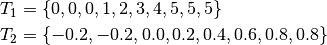
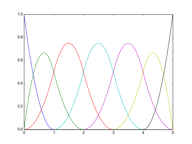
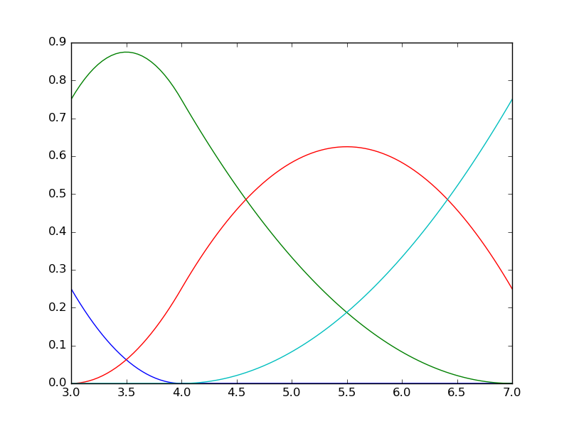
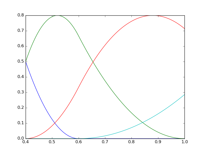
The j-th B-Spline of order is defined by the recurrence relation:

where,
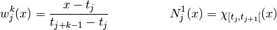
for  and
and  .
.
We note some important properties of a B-splines basis:
- B-splines are piecewise polynomial of degree
 ,
, - Compact support; the support of
 is contained in
 ![\left[ t_j, t_{j+k} \right]](../_images/math/123ad99deea307dd580b2eca671cf82407cd64a4.png) ,
, - If
![x \in~ ] t_j,t_{j+1} [](../_images/math/3e1d714facac1f93fbb78d5073622c19a234be42.png) , then only the B-splines
, then only the B-splines  are non vanishing at
  ,
, - Positivity:
![\forall j \in \{1,\cdots,n \}~~N_j(x) >0, ~~\forall x \in ] t_j, t_{j+k} [](../_images/math/e247cddc2012ac7fc0a6c66de300533eb5e27dc3.png) ,
, - Partition of unity
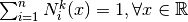 ,
, - Local linear independence,
- If a knot
 has a multiplicity
  then the B-spline is
  at .
at .
Knots vector families
There are two kind of knots vectors, called clamped and unclamped. Both families contains uniform and non-uniform sequences.
The following are examples of such knots vectors
- Clamped knots (open knots vector)
- uniform

- non-uniform
- Unclamped knots
- uniform
- non-uniform
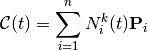
B-Spline curve
The B-spline curve in  associated to knots vector and the control polygon
  is defined by :
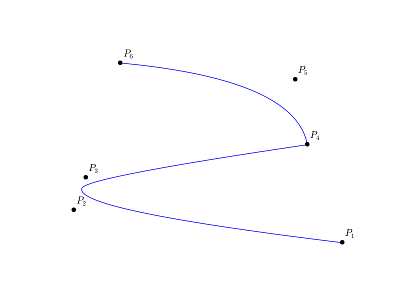
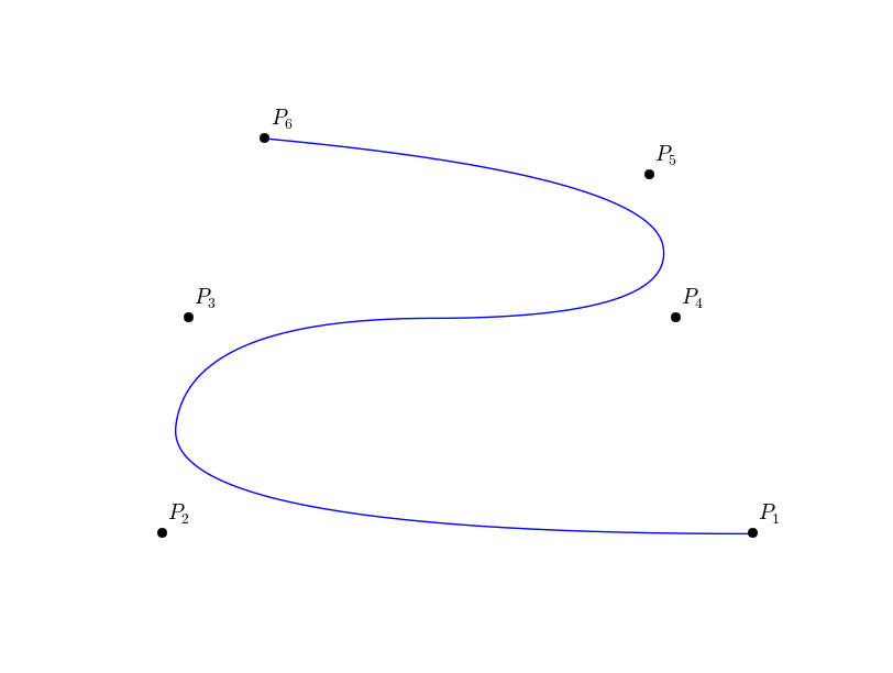
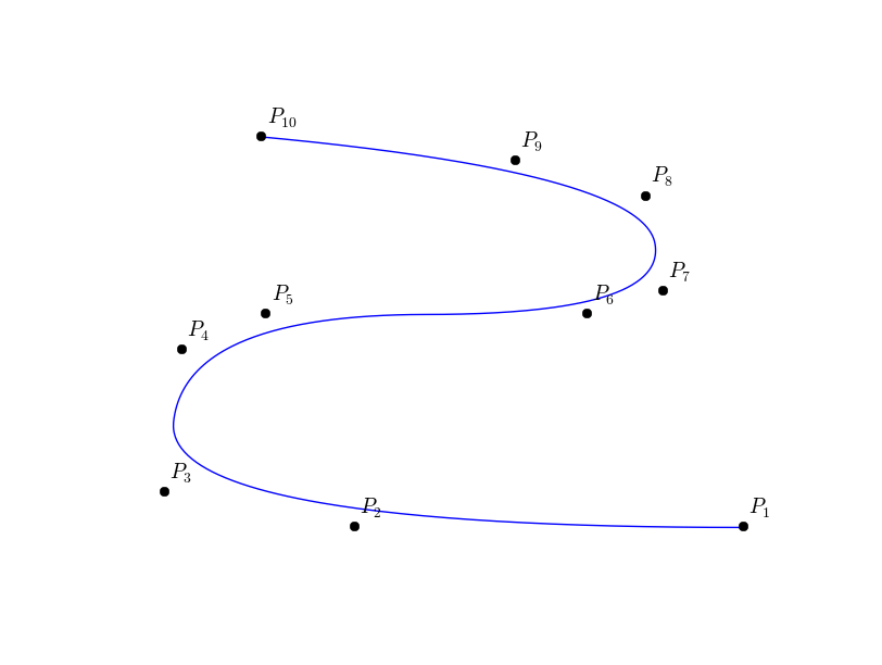
In (Fig. ref{figBSplineCurve}), we give an example of a quadratic B-Spline curve, and its corresponding knot vector and control points.
We have the following properties for a B-spline curve:
- If
 , then
  is just a B’ezier-curve,
 - is a piecewise polynomial curve,
- The curve interpolates its extremas if the associated multiplicity of the first and the last knot are maximum (i.e. equal to ), i.e. open knot vector,
- Invariance with respect to affine transformations,
- Strong convex-hull property:
if  , then
  is inside the convex-hull associated to the control points
  ,
,
- Local modification : moving the
 control point
  affects , only in the interval
 ![[t_i,t_{i+k}]](../_images/math/0ce0f55484121b1799699bb54757a0781a2914ac.png) ,
, - The control polygon approaches the behavior of the curve.
Note
In order to model a singular curve, we can use multiple control points :  .
.
Multivariate tensor product splines
Let us consider  knot vectors
  . For simplicity, we consider that these knot vectors are open, which means that knots on each side are duplicated so that the spline is interpolating on the boundary, and of bounds
  and
and  . In the sequel we will use the notation
 ![I=[0,1]](../_images/math/1ea1a67b54445a981ff544b1de542bf7525cd491.png) .
Each knot vector
.
Each knot vector  , will generate a basis for a Schoenberg space,
  . The tensor product of all these spaces is also a Schoenberg space, namely
  , where
  . The cube
 ![\mathcal{P}=I^d=[0,1]^d](../_images/math/3c47cd1746b54679c6db709e271167d2b7907d31.png) , will be referred to as a patch.
, will be referred to as a patch.
The basis for is defined by a tensor product :
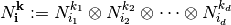
where,  .
.
A typical cell from  is a cube of the form :
 ![Q_{\mathbf{i}}=[\xi_{i_1}, \xi_{i_1+1}] \otimes \cdots \otimes [\xi_{i_d}, \xi_{i_d+1}]](../_images/math/83ca350a4ae0007515aecc041132cb71ed522881.png) .
.
Deriving a B-spline curve
The derivative of a B-spline curve is obtained as:

where  , and
, and  are generated using the knot vector
  , which is obtained from
  by reducing by one the multiplicity of the first and the last knot (in the case of open knot vector), i.e. by removing the first and the last knot.
More generally, by introducing the B-splines family  generated by the knots vector
  obtained from by removing the first and the last knot
  times, we have the following result:
proposition
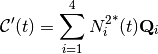
The  derivative of the curve is given by
where, for 
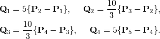
By denoting  and
and  the first and second derivative of the B-spline curve , it is easy to show that:
We have,
 ,
, ,
, ,
, .
.
Example
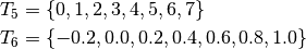
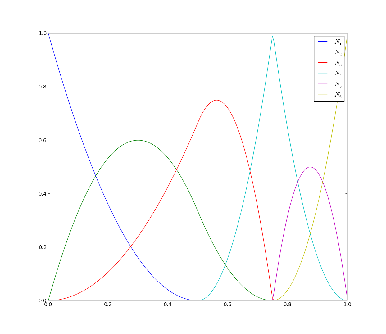
Let us consider the quadratic B-spline curve associated to the knots vector  and the control points
  :
:
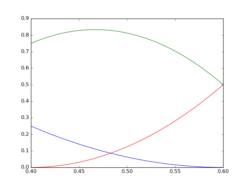
we have,
where
The B-splines 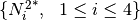 are associated to the knot vector
 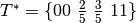 .
.
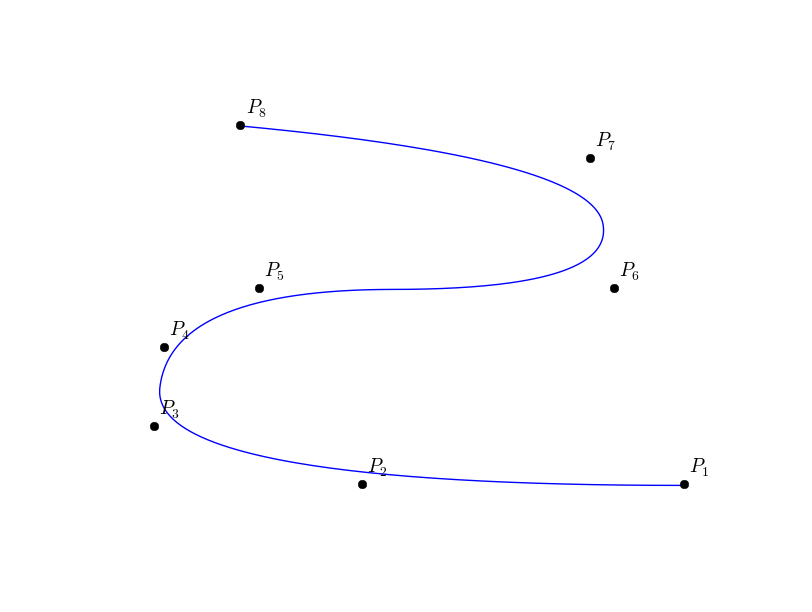
Fundamental geometric operations
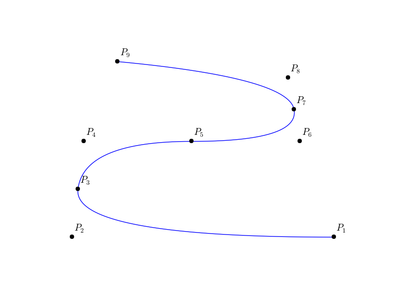
By inserting new knots into the knot vector, we add new control points without changing the shape of the B-Spline curve. This can be done using the DeBoor algorithm [dB01]. We can also elevate the degree of the B-Spline family and keep unchanged the curve [HHM05]. In (Fig. ref{refinement_curve_B_Spline}), we apply these algorithms on a quadratic B-Spline curve and we show the position of the new control points.
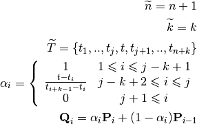
Knot insertion
After modification, we denote by  the new parameters.
  are the new control points.
One can insert a new knot  , where
  . For this purpose we use the DeBoor algorithm [dB01]:
Many other algorithms exist, like blossoming for fast insertion algorithm. For more details about this topic, we refer to [NT93].
Order elevation
We can elevate the order of the basis, without changing the curve. Several algorithms exist for this purpose. We used the one by Huang et al. [PP91], [HHM05].
A quadratic B-spline curve and its control points. The knot vector is 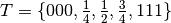 .
.
The curve after a h-refinement by inserting the knots  while the degree is kept equal to
  .
.
The curve after a p-refinement, the degree was raised by (using cubic B-splines).
The curve after duplicating the multiplicity of the internal knots  ,
this leads to a B’ezier description. We can then, split the curve into
,
this leads to a B’ezier description. We can then, split the curve into  pieces (sub-domains), each one will corresponds to a quadratic B’ezier curve.
Translation
Rotation
Todo
not yet available
Scaling
Todo
not yet available
References
| [dB01] | (1, 2) C. de Boor. A Practical Guide to Splines. Applied Mathematical Sciences. Springer New York, 2001. ISBN 9780387953663. URL: https://books.google.de/books?id=m0QDJvBI_ecC. |
| [Far02] | G. Farin. Curves and surfaces for CAGD: a practical guide. Morgan Kaufmann Pub. Inc., San Francisco, CA, USA, 2002. ISBN 1-55860-737-4. |
| [HHM05] | (1, 2) Qi-Xing Huang, Shi-Min Hu, and Ralph R. Martin. Fast degree elevation and knot insertion for b-spline curves. Computer Aided Geometric Design, 22(2):183 – 197, 2005. URL: http://www.sciencedirect.com/science/article/B6TYN-4DXBTHR-2/2/d5b3eec2f4c230c8051623c1c000beae, doi:DOI: 10.1016/j.cagd.2004.11.001. |
| [LP95] | W. Tiller L. Piegl. The NURBS Book. Springer-Verlag, Berlin, Heidelberg, 1995. second ed. |
| [NT93] | Goldman R. N. and Lyche T. Knot Insertion and Deletion Algorithms for B-Spline Curves and Surfaces. SIAM, Philadelphia, USA, 1993. ISBN 9780898713060. |
| [PP91] | Hartmut Prautzsch and Bruce Piper. A fast algorithm to raise the degree of spline curves. Comput. Aided Geom. Des., 8:253–265, October 1991. URL: http://portal.acm.org/citation.cfm?id=124930.124932, doi:10.1016/0167-8396(91)90015-4. |